Step-by-Step Tutorial to Constructing Your First Machine Studying Mannequin

Picture by pch.vector on Freepik

Hello everybody! I’m certain you might be studying this text as a result of you have an interest in a machine-learning mannequin and wish to construct one.

You’ll have tried to develop machine studying fashions earlier than or you might be fully new to the idea. Regardless of your expertise, this text will information you thru the perfect practices for creating machine studying fashions.

On this article, we’ll develop a Buyer Churn prediction classification mannequin following the steps under:

1. Enterprise Understanding
2. Information Assortment and Preparation

• Amassing Information
• Exploratory Information Evaluation (EDA) and Information Cleansing
• Function Choice

3. Constructing the Machine Studying Mannequin

• Selecting the Proper Mannequin
• Splitting the Information
• Coaching the Mannequin
• Mannequin Analysis

4. Mannequin Optimization

5. Deploying the Mannequin

Let’s get into it if you’re enthusiastic about constructing your first machine studying mannequin.

Understanding the Fundamentals

 
Earlier than we get into the machine studying mannequin growth, let’s briefly clarify machine studying, the varieties of machine studying, and some terminologies we’ll use on this article.

First, let’s focus on the varieties of machine studying fashions we are able to develop. 4 essential varieties of Machine Studying typically developed are:

• Supervised Machine Studying is a machine studying algorithm that learns from labeled datasets. Based mostly on the proper output, the mannequin learns from the sample and tries to foretell the brand new knowledge. There are two classes in Supervised Machine Studying: Classification (Class prediction) and Regression (Numerical prediction).
• Unsupervised Machine Studying is an algorithm that tries to seek out patterns in knowledge with out course. Not like supervised machine studying, the mannequin is just not guided by label knowledge. This kind has two frequent classes: Clustering (Information Segmentation) and Dimensionality Discount (Function Discount).
• Semi-supervised machine studying combines the labeled and unlabeled datasets, the place the labeled dataset guides the mannequin in figuring out patterns within the unlabeled knowledge. The only instance is a self-training mannequin that may label the unlabeled knowledge based mostly on a labeled knowledge sample.
• Reinforcement Studying is a machine studying algorithm that may work together with the atmosphere and react based mostly on the motion (getting a reward or punishment). It will maximize the end result with the rewards system and keep away from dangerous outcomes with punishment. An instance of this mannequin utility is the self-driving automobile.

You additionally have to know just a few terminologies to develop a machine-learning mannequin:

• Options: Enter variables used to make predictions in a machine studying mannequin.
• Labels: Output variables that the mannequin is making an attempt to foretell.
• Information Splitting: The method of information separation into totally different units.
• Coaching Set: Information used to coach the machine studying mannequin.
• Check Set: Information used to judge the efficiency of the educated mannequin.
• Validation Set: Information use used in the course of the coaching course of to tune hyperparameters
• Exploratory Information Evaluation (EDA): The method of analyzing and visualizing datasets to summarize their info and uncover patterns.
• Fashions: The result of the Machine Studying course of. They’re the mathematical illustration of the patterns and relationships inside the knowledge.
• Overfitting: Happens when the mannequin is generalized too effectively and learns the info noise. The mannequin can predict effectively within the coaching however not within the check set.
• Underfitting: When a mannequin is just too easy to seize the underlying patterns within the knowledge. The mannequin efficiency in coaching and check units may very well be higher.
• Hyperparameters: Configuration settings are used to tune the mannequin and are set earlier than coaching begins.
• Cross-validation: a method for evaluating the mannequin by partitioning the unique pattern into coaching and validation units a number of instances.
• Function Engineering: Utilizing area information to get new options from uncooked knowledge.
• Mannequin Coaching: The method of studying the parameters of a mannequin utilizing the coaching knowledge.
• Mannequin Analysis: Assessing the efficiency of a educated mannequin utilizing machine studying metrics like accuracy, precision, and recall.
• Mannequin Deployment: Making a educated mannequin out there in a manufacturing atmosphere.

With all this primary information, let’s be taught to develop our first machine-learning mannequin.
 

1. Enterprise Understanding

 
Earlier than any machine studying mannequin growth, we should perceive why we should develop the mannequin. That’s why understanding what the enterprise desires is important to make sure the mannequin is legitimate.
Enterprise understanding often requires a correct dialogue with the associated stakeholders. Nonetheless, since this tutorial doesn’t have enterprise customers for the machine studying mannequin, we assume the enterprise wants ourselves.

As said beforehand, we’d develop a Buyer Churn prediction mannequin. On this case, the enterprise must keep away from additional churn from the corporate and desires to take motion for the shopper with a excessive chance of churning.
With the above enterprise necessities, we want particular metrics to measure whether or not the mannequin performs effectively. There are a lot of measurements, however I suggest utilizing the Recall metric.

In financial values, it could be extra useful to make use of Recall, because it tries to reduce the False Unfavourable or lower the quantity of prediction that was not churning whereas it’s churning. After all, we are able to attempt to intention for stability through the use of the F1 metric.

With that in thoughts, let’s get into the primary a part of our tutorial.
 

2. Information Assortment and Preparation

Information Assortment

Information is the center of any machine studying undertaking. With out it, we are able to’t have a machine studying mannequin to coach. That’s why we want high quality knowledge with correct preparation earlier than we enter them into the machine studying algorithm.

In a real-world case, clear knowledge doesn’t come simply. Typically, we have to acquire it by way of purposes, surveys, and lots of different sources earlier than storing it in knowledge storage. Nonetheless, this tutorial solely covers amassing the dataset as we use the present clear knowledge.

In our case, we’d use the Telco Buyer Churn knowledge from the Kaggle. It’s open-source classification knowledge concerning buyer historical past within the telco trade with the churn label.
 

Exploratory Information Evaluation (EDA) and Information Cleansing

 
Let’s begin by reviewing our dataset. I assume the reader already has primary Python information and may use Python packages of their pocket book. I additionally based mostly the tutorial on Anaconda atmosphere distribution to make issues simpler.

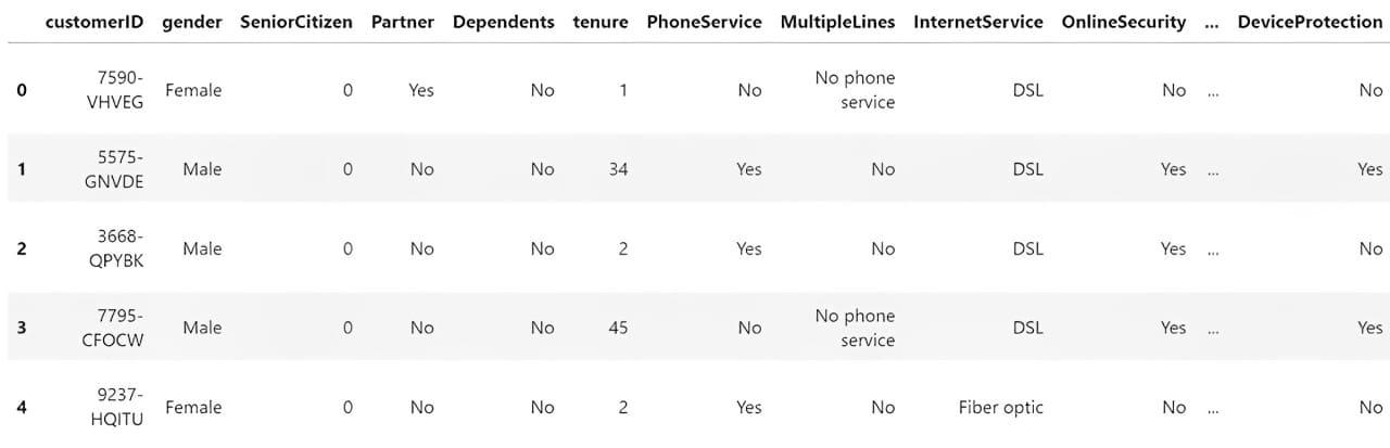
To know the info now we have, we have to load it right into a Python bundle for knowledge manipulation. Probably the most well-known one is the Pandas Python bundle, which we’ll use. We are able to use the next code to load and assessment the CSV knowledge.

import pandas as pd

df = pd.read_csv('WA_Fn-UseC_-Telco-Buyer-Churn.csv')
df.head()

Subsequent, we’d discover the info to know our dataset. Listed below are just a few actions that we’d carry out for the EDA course of.

1. Inspecting the options and the abstract statistics.
2. Checks for lacking values within the options.
3. Analyze the distribution of the label (Churn).
4. Plots histograms for numerical options and bar plots for categorical options.
5. Plots a correlation heatmap for numerical options.
6. Makes use of field plots to establish distributions and potential outliers.

First, we’d examine the options and abstract statistics. With Pandas, we are able to see our dataset options utilizing the next code.

# Get the essential details about the dataset
df.information()

Output>>

RangeIndex: 7043 entries, 0 to 7042
Information columns (whole 21 columns):
 #   Column            Non-Null Rely  Dtype  
---  ------            --------------  -----  
 0   customerID        7043 non-null   object 
 1   gender            7043 non-null   object 
 2   SeniorCitizen     7043 non-null   int64  
 3   Accomplice           7043 non-null   object 
 4   Dependents        7043 non-null   object 
 5   tenure            7043 non-null   int64  
 6   PhoneService      7043 non-null   object 
 7   MultipleLines     7043 non-null   object 
 8   InternetService   7043 non-null   object 
 9   OnlineSecurity    7043 non-null   object 
 10  OnlineBackup      7043 non-null   object 
 11  DeviceProtection  7043 non-null   object 
 12  TechSupport       7043 non-null   object 
 13  StreamingTV       7043 non-null   object 
 14  StreamingMovies   7043 non-null   object 
 15  Contract          7043 non-null   object 
 16  PaperlessBilling  7043 non-null   object 
 17  PaymentMethod     7043 non-null   object 
 18  MonthlyCharges    7043 non-null   float64
 19  TotalCharges      7043 non-null   object 
 20  Churn             7043 non-null   object 
dtypes: float64(1), int64(2), object(18)
reminiscence utilization: 1.1+ MB

We might additionally get the dataset abstract statistics with the next code.

# Get the numerical abstract statistics of the dataset
df.describe()

# Get the explicit abstract statistics of the dataset
df.describe(exclude="quantity")

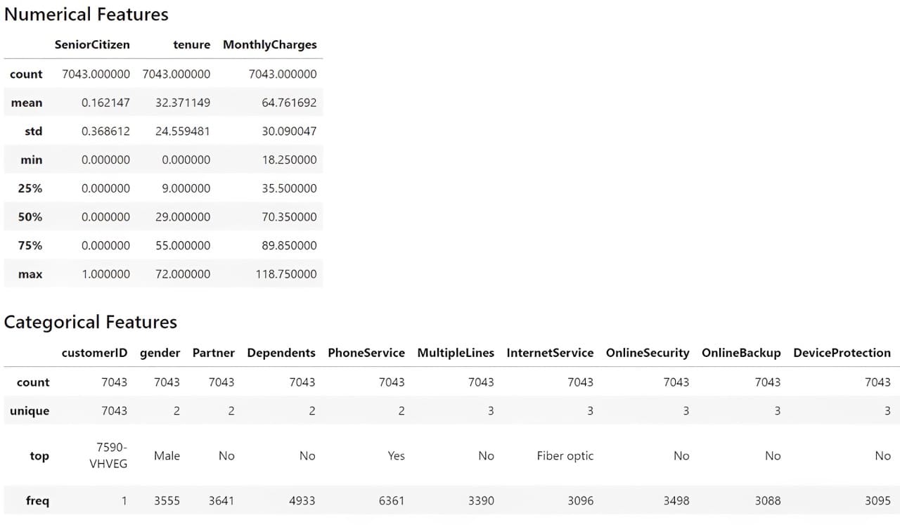
From the data above, we perceive that now we have 19 options with one goal function (Churn). The dataset accommodates 7043 rows, and most datasets are categorical.

Let’s examine for the lacking knowledge.

# Verify for lacking values
print(df.isnull().sum())

Output>>
Lacking Values:
customerID          0
gender              0
SeniorCitizen       0
Accomplice             0
Dependents          0
tenure              0
PhoneService        0
MultipleLines       0
InternetService     0
OnlineSecurity      0
OnlineBackup        0
DeviceProtection    0
TechSupport         0
StreamingTV         0
StreamingMovies     0
Contract            0
PaperlessBilling    0
PaymentMethod       0
MonthlyCharges      0
TotalCharges        0
Churn               0

Our dataset doesn’t include lacking knowledge, so we don’t have to carry out any lacking knowledge therapy exercise.
Then, we’d examine the goal variable to see if now we have an imbalance case.

print(df['Churn'].value_counts())

Output>>
Distribution of Goal Variable:
No     5174
Sure    1869

There’s a slight imbalance, as solely near 25% of the churn happens in comparison with the non-churn instances.

Let’s additionally see the distribution of the opposite options, beginning with the numerical options. Nonetheless, we’d additionally rework the TotalCharges function right into a numerical column, as this function ought to be numerical fairly than a class. Moreover, the SeniorCitizen function ought to be categorical in order that I might rework it into strings. Additionally, because the Churn function is categorical, we’d develop new options that present it as a numerical column.

import numpy as np
df['TotalCharges'] = df['TotalCharges'].exchange('', np.nan)
df['TotalCharges'] = pd.to_numeric(df['TotalCharges'], errors="coerce").fillna(0)

df['SeniorCitizen'] = df['SeniorCitizen'].astype('str')

df['ChurnTarget'] = df['Churn'].apply(lambda x: 1 if x=='Sure' else 0)

df['ChurnTarget'] = df['Churn'].apply(lambda x: 1 if x=='Sure' else 0)

num_features = df.select_dtypes('quantity').columns
df[num_features].hist(bins=15, figsize=(15, 6), structure=(2, 5))

We might additionally present categorical function plotting apart from the customerID, as they’re identifiers with distinctive values.

import matplotlib.pyplot as plt
# Plot distribution of categorical options
cat_features = df.drop('customerID', axis =1).select_dtypes(embody="object").columns

plt.determine(figsize=(20, 20))
for i, col in enumerate(cat_features, 1):
    plt.subplot(5, 4, i)
    df[col].value_counts().plot(variety='bar')
    plt.title(col)

We then would see the correlation between numerical options with the next code.

import seaborn as sns

# Plot correlations between numerical options
plt.determine(figsize=(10, 8))
sns.heatmap(df[num_features].corr())
plt.title('Correlation Heatmap')

The correlation above relies on the Pearson Correlation, a linear correlation between one function and the opposite. We are able to additionally carry out correlation evaluation to categorical evaluation with Cramer’s V. To make the evaluation simpler, we’d set up Dython Python bundle that might assist our evaluation.

As soon as the bundle is put in, we’ll carry out the correlation evaluation with the next code.

from dython.nominal import associations

# Calculate the Cramer’s V and correlation matrix
assoc = associations(df[cat_features], nominal_columns="all", plot=False)
corr_matrix = assoc['corr']

# Plot the heatmap
plt.determine(figsize=(14, 12))
sns.heatmap(corr_matrix)

Lastly, we’d examine the numerical outlier with a field plot based mostly on the Interquartile Vary (IQR).

# Plot field plots to establish outliers
plt.determine(figsize=(20, 15))
for i, col in enumerate(num_features, 1):
    plt.subplot(4, 4, i)
    sns.boxplot(y=df[col])
    plt.title(col)

From the evaluation above, we are able to see that we must always tackle no lacking knowledge or outliers. The following step is to carry out function choice for our machine studying mannequin, as we solely need the options that affect the prediction and are viable within the enterprise.

Function Choice

There are a lot of methods to carry out function choice, often completed by combining enterprise information and technical utility. Nonetheless, this tutorial will solely use the correlation evaluation now we have completed beforehand to make the function choice.

First, let’s choose the numerical options based mostly on the correlation evaluation.

goal="ChurnTarget"
num_features = df.select_dtypes(embody=[np.number]).columns.drop(goal)

# Calculate correlations
correlations = df[num_features].corrwith(df[target])

# Set a threshold for function choice
threshold = 0.3
selected_num_features = correlations[abs(correlations) > threshold].index.tolist()

You’ll be able to mess around with the edge later to see if the function choice impacts the mannequin’s efficiency. We might additionally carry out the function choice into the explicit options.

categorical_target="Churn"

assoc = associations(df[cat_features], nominal_columns="all", plot=False)
corr_matrix = assoc['corr']

threshold = 0.3
selected_cat_features = corr_matrix[corr_matrix.loc[categorical_target] > threshold ].index.tolist()

del selected_cat_features[-1]

Then, we’d mix all the chosen options with the next code.

selected_features = []
selected_features.prolong(selected_num_features)
selected_features.prolong(selected_cat_features)

print(selected_features)

Output>>
['tenure',
 'InternetService',
 'OnlineSecurity',
 'TechSupport',
 'Contract',
 'PaymentMethod']

In the long run, now we have six options that might be used to develop the shopper churn machine studying mannequin.
 

3. Constructing the Machine Studying Mannequin

Selecting the Proper Mannequin

There are a lot of issues to picking an acceptable mannequin for machine studying growth, however it at all times is dependent upon the enterprise wants. Just a few factors to recollect:

1. The use case drawback. Is it supervised or unsupervised, or is it classification or regression? Is it Multiclass or Multilabel? The case drawback would dictate which mannequin can be utilized.
2. The info traits. Is it tabular knowledge, textual content, or picture? Is the dataset measurement huge or small? Did the dataset include lacking values? Relying on the dataset, the mannequin we select may very well be totally different.
3. How straightforward is the mannequin to be interpreted? Balancing interpretability and efficiency is important for the enterprise.

As a thumb rule, beginning with a less complicated mannequin as a benchmark is commonly finest earlier than continuing to a posh one. You’ll be able to learn my earlier article concerning the easy mannequin to know what constitutes a easy mannequin.

For this tutorial, let’s begin with linear mannequin Logistic Regression for the mannequin growth.
 

Splitting the Information

The following exercise is to separate the info into coaching, check, and validation units. The aim of information splitting throughout machine studying mannequin coaching is to have a knowledge set that acts as unseen knowledge (real-world knowledge) to judge the mannequin unbias with none knowledge leakage.

To separate the info, we’ll use the next code:

from sklearn.model_selection import train_test_split

goal="ChurnTarget" 

X = df[selected_features]
y = df[target]

cat_features = X.select_dtypes(embody=['object']).columns.tolist()
num_features = X.select_dtypes(embody=['number']).columns.tolist()

#Splitting knowledge into Prepare, Validation, and Check Set
X_train_val, X_test, y_train_val, y_test = train_test_split(X, y, test_size=0.2, random_state=42, stratify=y)

X_train, X_val, y_train, y_val = train_test_split(X_train_val, y_train_val, test_size=0.25, random_state=42, stratify=y_train_val)

Within the above code, we cut up the info into 60% of the coaching dataset and 20% of the check and validation set. As soon as now we have the dataset, we’ll practice the mannequin.
 

Coaching the Mannequin

As talked about, we’d practice a Logistic Regression mannequin with our coaching knowledge. Nonetheless, the mannequin can solely settle for numerical knowledge, so we should preprocess the dataset. This implies we have to rework the explicit knowledge into numerical knowledge.

For finest observe, we additionally use the Scikit-Study pipeline to include all of the preprocessing and modeling steps. The next code lets you do this.

from sklearn.compose import ColumnTransformer
from sklearn.pipeline import Pipeline
from sklearn.preprocessing import OneHotEncoder
from sklearn.linear_model import LogisticRegression
# Put together the preprocessing step
preprocessor = ColumnTransformer(
    transformers=[
        ('num', 'passthrough', num_features),
        ('cat', OneHotEncoder(), cat_features)
    ])

pipeline = Pipeline(steps=[
    ('preprocessor', preprocessor),
    ('classifier', LogisticRegression(max_iter=1000))
])

# Prepare the logistic regression mannequin
pipeline.match(X_train, y_train)

The mannequin pipeline would appear to be the picture under.

The Scikit-Study pipeline would settle for the unseen knowledge and undergo all of the preprocessing steps earlier than getting into the mannequin. After the mannequin is completed coaching, let’s consider our mannequin end result.
 

Mannequin Analysis

As talked about, we’ll consider the mannequin by specializing in the Recall metrics. Nonetheless, the next code reveals all the essential classification metrics.

from sklearn.metrics import classification_report

# Consider on the validation set
y_val_pred = pipeline.predict(X_val)
print("Validation Classification Report:n", classification_report(y_val, y_val_pred))

# Consider on the check set
y_test_pred = pipeline.predict(X_test)
print("Check Classification Report:n", classification_report(y_test, y_test_pred))

As we are able to see from the Validation and Check knowledge, the Recall for churn (1) is just not the perfect. That’s why we are able to optimize the mannequin to get the perfect end result.
 

4. Mannequin Optimization

 
We at all times have to give attention to the info to get the perfect end result. Nonetheless, optimizing the mannequin may additionally result in higher outcomes. This is the reason we are able to optimize our mannequin. One method to optimize the mannequin is by way of hyperparameter optimization, which checks all mixtures of those mannequin hyperparameters to seek out the perfect one based mostly on the metrics.

Each mannequin has a set of hyperparameters we are able to set earlier than coaching it. We name hyperparameter optimization the experiment to see which mixture is the perfect. To try this, we are able to use the next code.

from sklearn.model_selection import GridSearchCV
# Outline the logistic regression mannequin inside a pipeline
pipeline = Pipeline(steps=[
    ('preprocessor', preprocessor),
    ('classifier', LogisticRegression(max_iter=1000))
])

# Outline the hyperparameters for GridSearchCV
param_grid = {
    'classifier__C': [0.1, 1, 10, 100],
    'classifier__solver': ['lbfgs', 'liblinear']
}

# Carry out Grid Search with cross-validation
grid_search = GridSearchCV(pipeline, param_grid, cv=5, scoring='recall')
grid_search.match(X_train, y_train)

# Greatest hyperparameters
print("Greatest Hyperparameters:", grid_search.best_params_)

# Consider on the validation set
y_val_pred = grid_search.predict(X_val)
print("Validation Classification Report:n", classification_report(y_val, y_val_pred))

# Consider on the check set
y_test_pred = grid_search.predict(X_test)
print("Check Classification Report:n", classification_report(y_test, y_test_pred))

The outcomes nonetheless don’t present the perfect recall rating, however that is anticipated as they’re solely the baseline mannequin. Let’s experiment with a number of fashions to see if the Recall efficiency improves. You’ll be able to at all times tweak the hyperparameter under.

from sklearn.tree import DecisionTreeClassifier
from sklearn.ensemble import RandomForestClassifier, GradientBoostingClassifier
from sklearn.svm import SVC
from xgboost import XGBClassifier
from lightgbm import LGBMClassifier
from sklearn.metrics import recall_score

# Outline the fashions and their parameter grids
fashions = {
    'Logistic Regression': {
        'mannequin': LogisticRegression(max_iter=1000),
        'params': {
            'classifier__C': [0.1, 1, 10, 100],
            'classifier__solver': ['lbfgs', 'liblinear']
        }
    },
    'Choice Tree': {
        'mannequin': DecisionTreeClassifier(),
        'params': {
            'classifier__max_depth': [None, 10, 20, 30],
            'classifier__min_samples_split': [2, 10, 20]
        }
    },
    'Random Forest': {
        'mannequin': RandomForestClassifier(),
        'params': {
            'classifier__n_estimators': [100, 200],
            'classifier__max_depth': [None, 10, 20]
        }
    },
    'SVM': {
        'mannequin': SVC(),
        'params': {
            'classifier__C': [0.1, 1, 10, 100],
            'classifier__kernel': ['linear', 'rbf']
        }
    },
    'Gradient Boosting': {
        'mannequin': GradientBoostingClassifier(),
        'params': {
            'classifier__n_estimators': [100, 200],
            'classifier__learning_rate': [0.01, 0.1, 0.2]
        }
    },
    'XGBoost': {
        'mannequin': XGBClassifier(use_label_encoder=False, eval_metric="logloss"),
        'params': {
            'classifier__n_estimators': [100, 200],
            'classifier__learning_rate': [0.01, 0.1, 0.2],
            'classifier__max_depth': [3, 6, 9]
        }
    },
    'LightGBM': {
        'mannequin': LGBMClassifier(),
        'params': {
            'classifier__n_estimators': [100, 200],
            'classifier__learning_rate': [0.01, 0.1, 0.2],
            'classifier__num_leaves': [31, 50, 100]
        }
    }
}

outcomes = []

# Prepare and consider every mannequin
for model_name, model_info in fashions.objects():
    pipeline = Pipeline(steps=[
        ('preprocessor', preprocessor),
        ('classifier', model_info['model'])
    ])
    
    grid_search = GridSearchCV(pipeline, model_info['params'], cv=5, scoring='recall')
    grid_search.match(X_train, y_train)
    
    # Greatest mannequin from Grid Search
    best_model = grid_search.best_estimator_
    
    # Consider on the validation set
    y_val_pred = best_model.predict(X_val)
    val_recall = recall_score(y_val, y_val_pred, pos_label=1)
    
    # Consider on the check set
    y_test_pred = best_model.predict(X_test)
    test_recall = recall_score(y_test, y_test_pred, pos_label=1)
    
    # Save outcomes
    outcomes.append({
        'mannequin': model_name,
        'best_params': grid_search.best_params_,
        'val_recall': val_recall,
        'test_recall': test_recall,
        'classification_report_val': classification_report(y_val, y_val_pred),
        'classification_report_test': classification_report(y_test, y_test_pred)
    })

# Plot the check recall scores
plt.determine(figsize=(10, 6))
model_names = [result['model'] for end in outcomes]
test_recalls = [result['test_recall'] for end in outcomes]
plt.barh(model_names, test_recalls, colour="skyblue")
plt.xlabel('Check Recall')
plt.title('Comparability of Check Recall for Completely different Fashions')
plt.present()

The recall end result has not modified a lot; even the baseline Logistic Regression appears the perfect. We must always return with a greater function choice if we wish a greater end result.

Nonetheless, let’s transfer ahead with the present Logistic Regression mannequin and attempt to deploy them.
 

5. Deploying the Mannequin

 
We’ve constructed our machine studying mannequin. After having the mannequin, the following step is to deploy it into manufacturing. Let’s simulate it utilizing a easy API.

First, let’s develop our mannequin once more and reserve it as a joblib object.

import joblib

best_params = {'classifier__C': 1, 'classifier__solver': 'lbfgs'}
logreg_model = LogisticRegression(C=best_params['classifier__C'], solver=best_params['classifier__solver'], max_iter=1000)

preprocessor = ColumnTransformer(
    transformers=[
        ('num', 'passthrough', num_features),
        ('cat', OneHotEncoder(), cat_features)

pipeline = Pipeline(steps=[
    ('preprocessor', preprocessor),
    ('classifier', logreg_model)
])

pipeline.match(X_train, y_train)

# Save the mannequin
joblib.dump(pipeline, 'logreg_model.joblib')

As soon as the mannequin object is prepared, we’ll transfer right into a Python script to create the API. However first, we have to set up just a few packages used for deployment.

pip set up fastapi uvicorn

We might not do it within the pocket book however in an IDE equivalent to Visible Studio Code. In your most popular IDE, create a Python script known as app.py and put the code under into the script.

from fastapi import FastAPI
from pydantic import BaseModel
import joblib
import numpy as np

# Load the logistic regression mannequin pipeline
mannequin = joblib.load('logreg_model.joblib')

# Outline the enter knowledge for mannequin
class CustomerData(BaseModel):
    tenure: int
    InternetService: str
    OnlineSecurity: str
    TechSupport: str
    Contract: str
    PaymentMethod: str

# Create FastAPI app
app = FastAPI()

# Outline prediction endpoint
@app.submit("/predict")
def predict(knowledge: CustomerData):
    # Convert enter knowledge to a dictionary after which to a DataFrame
    input_data = {
        'tenure': [data.tenure],
        'InternetService': [data.InternetService],
        'OnlineSecurity': [data.OnlineSecurity],
        'TechSupport': [data.TechSupport],
        'Contract': [data.Contract],
        'PaymentMethod': [data.PaymentMethod]
    }
   
    import pandas as pd
    input_df = pd.DataFrame(input_data)
   
    # Make a prediction
    prediction = mannequin.predict(input_df)
   
    # Return the prediction
    return {"prediction": int(prediction[0])}

if __name__ == "__main__":
    import uvicorn
    uvicorn.run(app, host="0.0.0.0", port=8000)

In your command immediate or terminal, run the next code.

With the code above, we have already got an API to simply accept knowledge and create predictions. Let’s attempt it out with the next code within the new terminal.

curl -X POST "http://127.0.0.1:8000/predict" -H "Content material-Sort: utility/json" -d "{"tenure": 72, "InternetService": "Fiber optic", "OnlineSecurity": "Sure", "TechSupport": "Sure", "Contract": "Two yr", "PaymentMethod": "Bank card (computerized)"}"

Output>>
{"prediction":0}

As you possibly can see, the API result’s a dictionary with prediction 0 (Not-Churn). You’ll be able to tweak the code even additional to get the specified end result.

Congratulation. You have got developed your machine studying mannequin and efficiently deployed it within the API.
 

Conclusion

 
We’ve discovered how you can develop a machine studying mannequin from the start to the deployment. Experiment with different datasets and use instances to get the sensation even higher. All of the code this text makes use of might be out there on my GitHub repository.
 
 

Cornellius Yudha Wijaya is a knowledge science assistant supervisor and knowledge author. Whereas working full-time at Allianz Indonesia, he likes to share Python and knowledge suggestions by way of social media and writing media. Cornellius writes on a wide range of AI and machine studying matters.