SVM One-Class Classifier For Anomaly Detection

Introduction

The One-Class Assist Vector Machine (SVM) is a variant of the standard SVM. It’s particularly tailor-made to detect anomalies. Its main intention is to find cases that notably deviate from the usual. Not like standard Machine Studying fashions centered on binary or multiclass classification, the one-class SVM focuses on outlier or novelty detection inside datasets. On this article, you’ll learn the way One-Class Assist Vector Machine (SVM) differs from conventional SVM. Additionally, you will learn the way OC-SVM works and how one can implement it. You’ll additionally find out about its hyperparameters. 

Studying Aims

• To know Anomalies
• Study One-class SVM
• Perceive the way it differs from conventional Assist Vector Machine (SVM)
• Hyperparameters of OC-SVM in Sklearn
• Find out how to detect Anomalies utilizing OC-SVM
• Use instances of One-class SVM

Understanding Anomalies

Anomalies are observations or cases that deviate considerably from a dataset’s regular conduct. These deviations can manifest in numerous varieties, resembling outliers, noise, errors, or sudden patterns. Anomalies are sometimes fascinating as a result of they could symbolize invaluable insights. They may present insights resembling figuring out fraudulent transactions, detecting tools malfunctions, or uncovering novel phenomena. Outlier and novelty detection determine anomalies and irregular or unusual observations.

Additionally Learn: An Finish-to-end Information on Anomaly Detection

One Class SVM

Introduction to Assist Vector Machines (SVMs)

Assist Vector Machines (SVMs) are a preferred supervised studying algorithm for classification and regression duties. SVMs work by discovering the optimum hyperplane that separates totally different courses in characteristic area whereas maximizing the margin between them. This hyperplane relies on a subset of coaching information factors referred to as assist vectors.

One-Class SVM vs Conventional SVM

• One-class SVMs symbolize a variant of the standard SVM algorithm primarily employed for outlier and novelty detection duties. Not like conventional SVMs, which deal with binary classification duties, One-Class SVM solely trains on information factors from a single class, generally known as the goal class. One-class SVM goals to be taught a boundary or determination operate that encapsulates the goal class in characteristic area, successfully modeling the traditional conduct of the information.

• Conventional SVMs intention to discover a determination boundary that maximizes the margin between totally different courses, permitting for optimum classification of recent information factors. Alternatively, One-Class SVM seeks to discover a boundary that encapsulates the goal class whereas minimizing the chance of together with outliers or novel cases outdoors this boundary.

• Conventional SVMs require labeled information with cases from a number of courses, making them appropriate for supervised classification duties. In distinction, a One-Class SVM permits software in situations the place solely information from the goal class is out there, making it well-suited for unsupervised anomaly detection and novelty detection duties.

Study Extra: One-Class Classification Utilizing Assist Vector Machines

They each differ of their comfortable margin formulations and the way in which they use them:

(Smooth margin in SVM is used to permit a point of misclassification)

One-class SVM goals to find a hyperplane with most margin inside the characteristic area by separating the mapped information from the origin. On a dataset Dn = {x1, . . . , xn} with xi ∈ X (xi is a characteristic) and n dimensions:

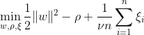
This equation represents the primal downside formulation for OC-SVM, the place w is the separating hyperplane, ρ is the offset from the origin, and ξi are slack variables. They permit for a comfortable margin however penalize violations ξi. A hyperparameter ν ∈ (0, 1] controls the impact of the slack variable and must be adjusted in line with want. The target is to attenuate the norm of w whereas penalizing deviations from the margin. Additional, this enables a fraction of the information to fall inside the margin or on the incorrect aspect of the hyperplane.

W.X + b =0 is the choice boundary, and the slack variables penalize deviations. 

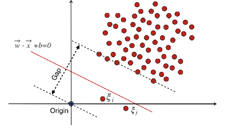
Conventional-Assist Vector Machines (SVM)

Conventional-Assist Vector Machines (SVM) use the comfortable margin formulation for misclassification errors. Or they use information factors that fall inside the margin or on the incorrect aspect of the choice boundary.

The place:

w is the load vector.

b is the bias time period. 

ξi are slack variables that enable for comfortable margin optimization.

C is the regularization parameter that controls the trade-off between maximizing the margin and minimizing the classification error. 

ϕ(xi) represents the characteristic mapping operate.

In conventional SVM, a supervised studying methodology that depends on class labels for separation incorporates slack variables to allow a sure stage of misclassification. SVM’s main goal is to separate information factors of distinct courses utilizing the choice boundary W.X + b = 0. The worth of slack variables varies relying on the situation of information factors: they’re set to 0 if the information factors are situated past the margins. If the information level resides inside the margin, the slack variables vary between 0 and 1, extending past the alternative margin if better than 1.

Each conventional SVMs and One-Class SVMs with comfortable margin formulations intention to attenuate the norm of the load vector. Nonetheless, they differ of their goals and the way they deal with misclassification errors or deviations from the choice boundary. Conventional SVMs optimize classification accuracy to keep away from overfitting, whereas One-Class SVMs deal with modeling the goal class and controlling the proportion of outliers or novel cases.

Additionally Learn: The A-Z Information to Assist Vector Machine

Necessary Hyperparameters in One-class SVM

• nu: This can be a essential hyperparameter in One-Class SVM, which controls the proportion of outliers allowed. It units an higher sure on the fraction of coaching errors and a decrease sure on the fraction of assist vectors. It sometimes ranges between 0 and 1, the place decrease values indicate a stricter margin and should seize fewer outliers, whereas greater values are extra permissive. The default worth is 0.5.
• kernel: The kernel operate determines the kind of determination boundary the SVM makes use of. Widespread selections embody ‘linear,’ ‘rbf’ (Gaussian radial foundation operate), ‘poly’ (polynomial), and ‘sigmoid.’ The ‘rbf’ kernel is commonly used as it will probably successfully seize advanced non-linear relationships.
• gamma: This can be a parameter for non-linear hyperplanes. It defines how a lot affect a single coaching instance has. The bigger the gamma worth, the nearer different examples have to be to be affected. This parameter is particular to the RBF kernel and is usually set to ‘auto,’ which defaults to 1 / n_features.
• kernel parameters (diploma, coef0): These parameters are for polynomial and sigmoid kernels. ‘diploma’ is the diploma of the polynomial kernel operate, and ‘coef0’ is the impartial time period within the kernel operate. Tuning these parameters could be needed for reaching optimum efficiency.
• tol: That is the stopping criterion. The algorithm stops when the duality hole is smaller than the tolerance. It’s a parameter that controls the tolerance for the stopping criterion.

Working Precept of One-Class SVM

Kernel Features in One-Class SVM

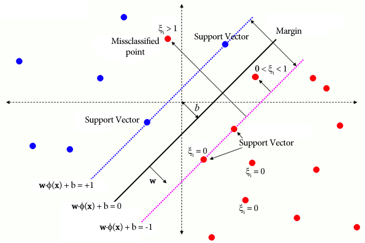
Kernel features play an important position in One-Class SVM by permitting the algorithm to function in higher-dimensional characteristic areas with out explicitly computing the transformations. In One-Class SVM, as in conventional SVMs, kernel features are used to measure the similarity between pairs of information factors within the enter area. Widespread kernel features utilized in One-Class SVM embody Gaussian (RBF), polynomial, and sigmoid kernels. These kernels map the unique enter area right into a higher-dimensional area, the place information factors turn into linearly separable or exhibit extra distinct patterns, facilitating studying. By selecting an applicable kernel operate and tuning its parameters, One-Class SVM can successfully seize advanced relationships and non-linear buildings within the information, enhancing its capability to detect anomalies or outliers.

In instances the place the information isn’t linearly separable, resembling when coping with advanced or overlapping patterns, Assist Vector Machines (SVMs) can make use of a Radial Foundation Operate (RBF) kernel to segregate outliers from the remainder of the information successfully. The RBF kernel transforms the enter information right into a higher-dimensional characteristic area that may be higher separated.

Margin and Assist Vectors

The idea of margin and assist vectors in One-Class SVM is just like that in conventional SVMs. The margin refers back to the area between the choice boundary (hyperplane) and the closest information factors from every class. In One-Class SVM, the margin represents the area the place a lot of the information factors belonging to the goal class lie. Maximizing the margin is essential for One-Class SVM because it helps generalize new information factors properly and improves the mannequin’s robustness. Assist vectors are the information factors that lie on or inside the margin and contribute to defining the choice boundary.

In One-Class SVM, assist vectors are the information factors from the goal class closest to the choice boundary. These assist vectors play a big position in figuring out the form and orientation of the choice boundary and, thus, within the total efficiency of the One-Class SVM mannequin. By figuring out the assist vectors, One-Class SVM successfully learns the illustration of the goal class within the characteristic area and constructs a choice boundary that encapsulates a lot of the information factors whereas minimizing the chance of together with outliers or novel cases.

How Anomalies Can Be Detected Utilizing One-Class SVM?

Detecting anomalies utilizing One-class SVM (Assist Vector Machine) by each novelty detection and outlier detection methods:

Outlier Detection

It entails figuring out observations within the coaching information that considerably deviate from the remainder, typically referred to as outliers. Estimators for outlier detection intention to suit the areas the place the coaching information is most concentrated, disregarding these deviant observations.

from sklearn.svm import OneClassSVM

from sklearn.datasets import load_wine

import matplotlib.pyplot as plt

import matplotlib.strains as mlines

from sklearn.inspection import DecisionBoundaryDisplay

# Load information

X = load_wine()["data"][:, [6, 9]]  # "banana"-shaped

# Outline estimators (One-Class SVM)

estimators_hard_margin = {

   "Arduous Margin OCSVM": OneClassSVM(nu=0.01, gamma=0.35),  # Very small nu for exhausting margin

}

estimators_soft_margin = {

   "Smooth Margin OCSVM": OneClassSVM(nu=0.25, gamma=0.35),  # Nu between 0 and 1 for comfortable margin

}

# Plotting setup

fig, axs = plt.subplots(1, 2, figsize=(12, 5))

colours = ["tab:blue", "tab:orange", "tab:red"]

legend_lines = []

# Arduous Margin OCSVM

ax = axs[0]

for shade, (title, estimator) in zip(colours, estimators_hard_margin.objects()):

   estimator.match(X)

   DecisionBoundaryDisplay.from_estimator(

       estimator,

       X,

       response_method="decision_function",

       plot_method="contour",

       ranges=[0],

       colours=shade,

       ax=ax,

   )

   legend_lines.append(mlines.Line2D([], [], shade=shade, label=title))

ax.scatter(X[:, 0], X[:, 1], shade="black")

ax.legend(handles=legend_lines, loc="higher middle")

ax.set(

   xlabel="flavanoids",

   ylabel="color_intensity",

   title="Arduous Margin Outlier detection (wine recognition)",

)

# Smooth Margin OCSVM

ax = axs[1]

legend_lines = []

for shade, (title, estimator) in zip(colours, estimators_soft_margin.objects()):

   estimator.match(X)

   DecisionBoundaryDisplay.from_estimator(

       estimator,

       X,

       response_method="decision_function",

       plot_method="contour",

       ranges=[0],

       colours=shade,

       ax=ax,

   )

   legend_lines.append(mlines.Line2D([], [], shade=shade, label=title))

ax.scatter(X[:, 0], X[:, 1], shade="black")

ax.legend(handles=legend_lines, loc="higher middle")

ax.set(

   xlabel="flavanoids",

   ylabel="color_intensity",

   title="Smooth Margin Outlier detection (wine recognition)",

)

plt.tight_layout()

plt.present()

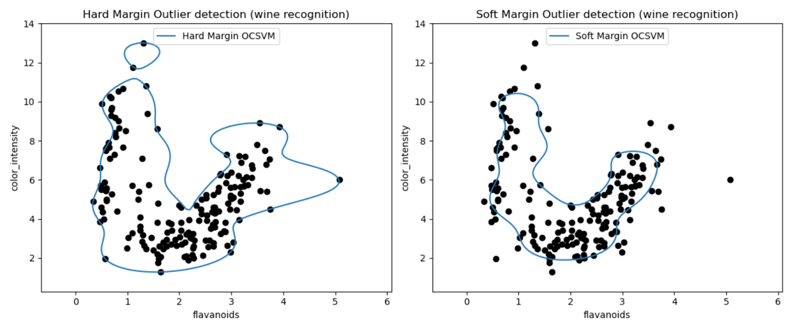
The plots enable us to visually examine the efficiency of the One-Class SVM fashions in detecting outliers within the Wine dataset.

By evaluating the outcomes of exhausting margin and comfortable margin One-Class SVM fashions, we are able to observe how the selection of margin setting (nu parameter) impacts outlier detection.

The exhausting margin mannequin with a really small nu worth (0.01) probably ends in a extra conservative determination boundary. It tightly wraps across the majority of the information factors and probably classifies fewer factors as outliers.

Conversely, the comfortable margin mannequin with a bigger nu worth (0.35) probably ends in a extra versatile determination boundary. Thus permitting for a wider margin and probably capturing extra outliers.

Novelty Detection

Alternatively, we apply it when the coaching information is free from outliers, and the purpose is to find out whether or not a brand new remark is uncommon, i.e., very totally different from identified observations. This newest remark right here is known as a novelty.

import numpy as np

from sklearn import svm

# Generate practice information

np.random.seed(30)

X = 0.3 * np.random.randn(100, 2)

X_train = np.r_[X + 2, X - 2]

# Generate some common novel observations

X = 0.3 * np.random.randn(20, 2)

X_test = np.r_[X + 2, X - 2]

# Generate some irregular novel observations

X_outliers = np.random.uniform(low=-4, excessive=4, measurement=(20, 2))

# match the mannequin

clf = svm.OneClassSVM(nu=0.1, kernel="rbf", gamma=0.1)

clf.match(X_train)

y_pred_train = clf.predict(X_train)

y_pred_test = clf.predict(X_test)

y_pred_outliers = clf.predict(X_outliers)

n_error_train = y_pred_train[y_pred_train == -1].measurement

n_error_test = y_pred_test[y_pred_test == -1].measurement

n_error_outliers = y_pred_outliers[y_pred_outliers == 1].measurement

import matplotlib.font_manager

import matplotlib.strains as mlines

import matplotlib.pyplot as plt

from sklearn.inspection import DecisionBoundaryDisplay

_, ax = plt.subplots()

# generate grid for the boundary show

xx, yy = np.meshgrid(np.linspace(-5, 5, 10), np.linspace(-5, 5, 10))

X = np.concatenate([xx.reshape(-1, 1), yy.reshape(-1, 1)], axis=1)

DecisionBoundaryDisplay.from_estimator(

   clf,

   X,

   response_method="decision_function",

   plot_method="contourf",

   ax=ax,

   cmap="PuBu",

)

DecisionBoundaryDisplay.from_estimator(

   clf,

   X,

   response_method="decision_function",

   plot_method="contourf",

   ax=ax,

   ranges=[0, 10000],

   colours="palevioletred",

)

DecisionBoundaryDisplay.from_estimator(

   clf,

   X,

   response_method="decision_function",

   plot_method="contour",

   ax=ax,

   ranges=[0],

   colours="darkred",

   linewidths=2,

)

s = 40

b1 = ax.scatter(X_train[:, 0], X_train[:, 1], c="white", s=s, edgecolors="okay")

b2 = ax.scatter(X_test[:, 0], X_test[:, 1], c="blueviolet", s=s, edgecolors="okay")

c = ax.scatter(X_outliers[:, 0], X_outliers[:, 1], c="gold", s=s, edgecolors="okay")

plt.legend(

   [mlines.Line2D([], [], shade="darkred"), b1, b2, c],

   [

       "learned frontier",

       "training observations",

       "new regular observations",

       "new abnormal observations",

   ],

   loc="higher left",

   prop=matplotlib.font_manager.FontProperties(measurement=11),

)

ax.set(

   xlabel=(

       f"error practice: {n_error_train}/200 ; errors novel common: {n_error_test}/40 ;"

       f" errors novel irregular: {n_error_outliers}/40"

   ),

   title="Novelty Detection",

   xlim=(-5, 5),

   ylim=(-5, 5),

)

plt.present()

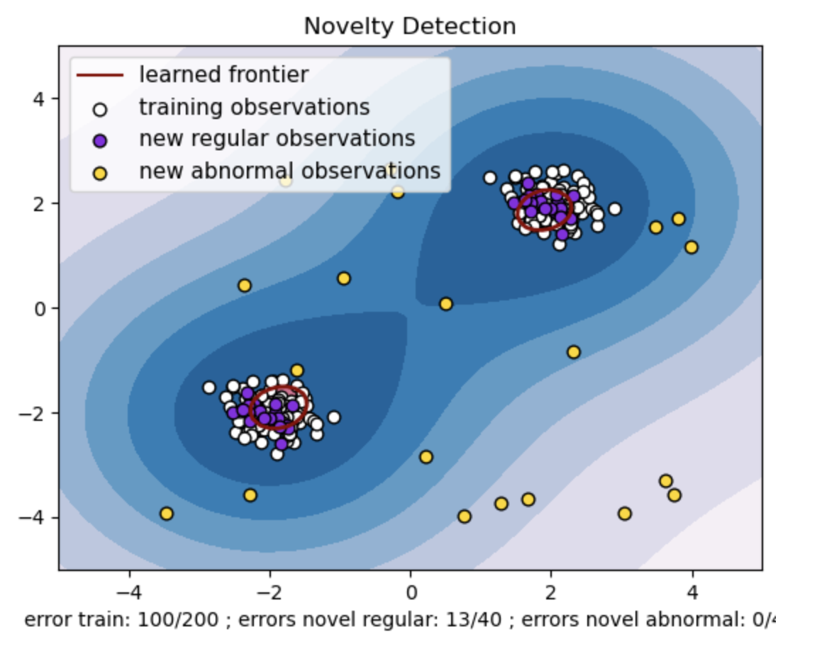
• Generate an artificial dataset with two clusters of information factors. Do that by producing them with a standard distribution round two totally different facilities: (2, 2) and (-2, -2) for practice and check information. Randomly generate twenty information factors uniformly inside a sq. area starting from -4 to 4 alongside each dimensions. These information factors symbolize irregular observations or outliers that deviate considerably from the traditional conduct noticed within the practice and check information.
• The discovered frontier refers back to the determination boundary discovered by the One-class SVM mannequin. This boundary separates the areas of the characteristic area the place the mannequin considers information factors to be regular from the outliers.
• The colour gradient from Blue to white within the contours represents the various levels of confidence or certainty that the One-Class SVM mannequin assigns to totally different areas within the characteristic area, with darker shades indicating greater confidence in classifying information factors as ‘regular.’ Darkish Blue signifies areas with a robust indication of being ‘regular’ in line with the mannequin’s determination operate. As the colour turns into lighter within the contour, the mannequin is much less positive about classifying information factors as ‘regular.’
• The plot visually represents how the One-class SVM mannequin can distinguish between common and irregular observations. The discovered determination boundary separates the areas of regular and irregular observations. One-class SVM for novelty detection proves its effectiveness in figuring out irregular observations in a given dataset.

For nu=0.5:

The “nu” worth in One-class SVM performs an important position in controlling the fraction of outliers tolerated by the mannequin. It immediately impacts the mannequin’s capability to determine anomalies and thus influences the prediction. We are able to see that the mannequin is permitting 100 coaching factors to be misclassified. A decrease worth of nu implies a stricter constraint on the allowed fraction of outliers. The selection of nu influences the mannequin’s efficiency in detecting anomalies. It additionally requires cautious tuning based mostly on the applying’s particular necessities and the dataset’s traits.

For gamma=0.5 and nu=0.5

In One-class SVM, the gamma hyperparameter represents the kernel coefficient for the ‘rbf’ kernel. This hyperparameter influences the form of the choice boundary and, consequently, impacts the mannequin’s predictive efficiency.

When gamma is excessive, a single coaching instance limits its affect to its instant neighborhood. This creates a extra localized determination boundary. Due to this fact, information factors have to be nearer to the assist vectors to belong to the identical class.

Conclusion

Using One-Class SVM for anomaly detection, utilizing outlier and novelty detection presents a sturdy resolution throughout numerous domains. This helps in situations the place labeled anomaly information is scarce or unavailable. Thus making it notably invaluable in real-world functions the place anomalies are uncommon and difficult to outline explicitly. Its use instances lengthen to numerous domains, resembling cybersecurity and fault prognosis, the place anomalies have penalties. Nevertheless, whereas One-Class SVM presents quite a few advantages, it’s essential to set the hyperparameters in line with the information to get higher outcomes, which may generally be tedious. 

Incessantly Requested Questions